The topics of trade entry risk analysis, and position risk management can become quite complex.

In this post, I want to share with you issues of trade entry risk analysis. At the bottom of the post are several videos I did which discuss the far more complex issues of position risk management.

It's not that evaluating trade entry risk is easier; it's just that entry risk is much simpler to analyze. Well, 3 of the aspects are simple.... The 4th one, however, is a beast....

4 Methods of FOREX Entry Risk Analysis

• The 2% Account Balance Method
• The Structural Analysis Method
• Static Pip Value Method
• Time Value Decay Analysis

Of note is that to this post, I have a companion video of the same title: 4 Methods of FOREX Entry Risk Analysis that puts all of this together from a different view point.

If you've come from watching that video, then press on here. However, if this is your starting point, I might suggest that you read through this before watching the video. Or, if you want, you can skip to the bottom of this post to watch that video now.

The primary factor in risk analysis

The primary factor in risk analysis — entry or position — deals with leverage, i.e. lot size as a function of account balance. Any discussion of risk needs to be prefaced with the leverage parameters being applied.

Leverage best practices are very simple: To trade 1 full lot of a currency pair you should have an account size of $10,000. This is because full lot size is based on $100,000 of currency.

The reason for that size of account (or $1,000 to trade a mini lot at $1 per pip) is because of the margin you must post just to sit at the table. In the U.S., and other major countries, you must have 5% margin, and not exceed 50 to 1 leverage.

Let's see how this works out on a currency pair trading at 1.2150.

The value of the trade is thus $121,500. 5% of that is $6,075, leaving $3,925 from your $10,000 account size as runway to trade at $10 per pip.

This means that you can lose 392 pips before getting a margin call.

Well, not exactly as that's where the leverage comes in.

If you're trading at 200 to 1, you'd hit the wood far before that. The $10 per pip is the result of the leverage of only trading 1 full lot against that 5% margin; without those restrictions it becomes a blood bath....

All of the examples in this post will be against a $1,000 account size, trading for $1 per pip on runway of $392, i.e. the same loss of 392 pips to hit margin (of $607 in the case of a mini lot worth $10,000 as opposed to the $100,000 full lot currency value).

I use the mini lot for ease of understanding because to calculate to full lot, or 10 full lots is simple. I don't advocate micro lots with $100 account sizes trading for $0.10 cents per lot. If you don't have $1,000 you shouldn't be trading these markets anyway....

So, 2% of the $1,000 bank is $20. Because it's a mini lot at $1 per pip, that 2% on bank is really 20 pips. Simple.

So, if you lose the first trade, i.e. $20/20pips, you're account balance is now $980.

To make another trade, you can now only risk 2% of $980: 19.6 pips. And now the calculations become complicated because each trade, whether a win or a loss, requires a different lot size for your trade entry.

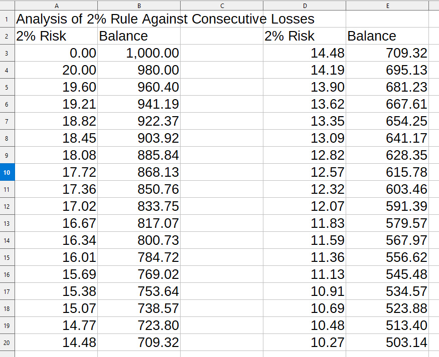
Analysis of 2% Rule Against Consecutive Losses

However, the major benefits of the 2% rule are 2 fold:

Benefits of Using 2% Risk Method

• De-leveraging after each loss enormously reduces the potential of losing your entire account.
• Increasing the lot size after each win by 2% of the account is called compounding, and, as Albert Einstein put it: "The most powerful invention I ever saw was compound interest."

Personal Note: I don't compound in the manner educational resources indicate it should be done. I take a different approach by using simple returns until certain criteria are met, and then I do a quantum jump in my lot size to the new value. This completely simplifies my process so that I can focus on the trade as opposed to all of the ancillary issues surrounding the trade.

This is a much more practical manner in which to view risk. The market doesn't care what 2% of your account is as that has absolutely no relevance to not only what the market is doing now, but what it has done in the past, or will do in the future. However, structure does.

The problem with determining a risk level from structural analysis is that structure tends to be a zone, or region, as opposed to a firm value.

Because of that, structures are up for interpretation, i.e. there are no 'rules' as to structural formation, or integrity to trading decisions.

We constantly see support and resistance lines as well as trend lines being drawn on a chart to represent structural boundaries. But what happens is that such a line drawn by one resource may be off 10 or more pips different in either or both directions than that drawn by another resource.

With so much variance, how do you teach this technique?

Well, sad to say: you can't teach it in a book, or video. This type of thing is experientially determined rather than through some rule. But if you don't have that experience, what are you supposed to do?

Well, you either have to run your account to the wood a few times to figure it all out for yourself, or find a mentor who understands how to present the principles in a manner that is logical, and will allow you to develop a 'sense' for such determinations.

I have a methodology which I feel is more mathematically based as to selecting these points or zones. But that still doesn't really provide much more accuracy than I might get just eyeballing the chart. This stuff just isn't exact enough to use in the manner that many educational resources suggest it is.

Simply following what you read or see in a video is just not going to provide you with that special trading 'sense' — that intuitive ability — to arrive at probabilistic determinations without doing any math. Or, you can do it with all the math, like I did, and not be any better able to trade using structural analysis than a 12 year old....

For me to discuss how I actually do this is beyond the scope of this post. The goal of the post is to discuss 'what' options you have for determining risk; not 'how' to implement such knowledge into your trading.

The long and the short of it is: structural analysis consists of evaluating price action congestion zones to determine the viability of that zone as a valid risk level.

As an additional caveat to consider with these structural zones is to note that a zone is determined by an indicator, i.e. a support or resistance line, or a trend line channel.

As I've discussed in many posts and videos: indicators only represent what has happened in the past and have absolutely no relevance to what is taking place in price action now, or could/might take place in the future.

Indicators are a complex subject, and can not be interpreted casually just because, for example, the fast ma crosses the slower ma, or some supposed 'support' level has been reached.

For a more detailed discussion of indicators you might be interested in my blog post The Myth of Using FOREX Currency Trading Indicators, or the videos listed below: Problems With Using Technical Analysis in FOREX Trading, and Fallacy of FOREX Trading Indicator Confluence.

This brings a consistency to your trading that basically eliminates risk as a metric in determining your trading efficiency.

By using this method of risk acceptance you completely simplify your whole aspect of your trade entry analysis. By eliminating risk considerations from your entry analysis you can focus on how to achieve the projected profit you have determined.

Of course, setting a static pip value is completely arbitrary, and has no correlation with past or present price action, structural component analysis, or any other function of price action. But then, that's the whole purpose of doing this type of static assignment in the first place....

I look at it this way: there is only 1 of 2 possible outcomes to a trade. Either you win, or you lose. Break even is not considered in this analysis.

You can not control how much a win will be, however, you can control how much you lose.

Well, you could rightly argue that any other form of trade entry risk mitigation controls the risk as well. And I would agree, except for the fact that all other methods of risk application are more subjective than objective.

Having a static pip value is simple, it creates consistency across metric analysis because it is lot size agnostic, and — because it eliminates the otherwise complex process of trade entry risk decision making — it frees the trader to focus on how to achieve the projected reward of the trade.

The following 2 diagram show calculations based on a starting bank balance of $10,000, winning 5% each month for 10 months, and then losing 8% for those 6 statistically likely trades in a row. The first diagram shows the results for compounding both gains and losses.

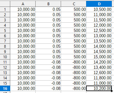
The second diagram shows the results for not compounding for either gains or losses, i.e. that static risk situation. As you can see by doing this, the results are $753.38 less in the account than by bi-directional compounding. That's a significant loss differential.

Even though using a static risk approach results in poorer overall trading performance, it's the method I prefer. I prefer it because it's simpler, and as I mentioned earlier in this section: it eliminates risk as a metric in determining your trading efficiency.

Having said that, I don't think it's appropriate for most folks. The general educational environment out there is so heavily oriented toward making things complex that it's tough to sort of 'go against the tide', so to say.

Besides, this post isn't meant to be a platform for me to suggest what you should do, but rather to simply point out the options you have for trade entry risk analysis.

I hope you enjoy my work enough that you follow through reading the additional posts I recommended, as well as watching the videos at the end of this post. As always, if you have any specific questions, throw me an email and I'll see if I can't give you a little more insight.

That all sounds pretty much like the closing music to a movie....

Yup, I'm basically done with this post. I've covered 3 basic ways of determining risk level for trade entry: 2%, Structure, and Static Pip. I mentioned that there was a 4th method, Time Value Decay Analysis.

You won't miss anything in your understanding of trade entry risk analysis by skipping over it, but you may get a headache trying to figure out what I'm talking about, and what relevance the discussion has with real time risk analysis. It's a beast, so if you're going to run through it, grab a coffee....

I'm going to approach this topic in broad strokes as the underlying statistical and probabilistic mathematics is stiff, to say the least. Thus, I'm going to have to shape things to match the outcome that I'm trying to describe.

I'll start off with the end by explaining what it all means, and then I'll get into all the gory details which support those conclusions.

I'm not going to go through the derivation of equations, but rather I'll discuss how the math suggests certain outcomes. And after all, that's really all you need to understand to implement some of the ideas.

This post is about evaluating risk for trade entry. But it's not the risk that decays with time: the longer the position remains on, the risk doesn't get less: it increases.

So, if the risk increases: what decreases? Yup, when the risk increases it means that the probability of the trade being successful decreases.

This is all you need to know!

If you are evaluating a trade entry situation and see that it's going to take a 'long' time for the trade to mature, then the risk will only increase with time, and thus that decay in potential profitability must be weighed against the increase in risk.

Of course, 'long' is subjective, and the 'how' of weighing decay of profitability against increasing risk over time is perplexing at best. I'll come back and discuss each of those issues after covering some of the following topics on the development of this theoretical conclusion.

To get there, however, will require a fantasy ride through stuff like the Physics of Brownian Motion, Black-Scholes Options Pricing Model Equation, and other arcane topics....

But, why, you ask? Well, by realizing that trading is supported theoretically, and that the better you understand those theoretical aspects, the more you will be able to make so-called intuitive decisions confidently.

Intuition is achieved by not only having a lot of information that is based on fact, but also in being able to trust the way your mind organizes that information, and then presents it to you as an actionable thought.

Developing this intuitive sense for trading through this type of quantitative analysis is only true, however, if you have an analytical mind.

If you function and learn better on an experiential basis in a more qualitative modality, then discussions like this just don't make sense. They can, in fact, be detrimental to your learning efforts.

Regardless: I press on....

This motion is named after the Scottish botanist Robert Brown (1773–1858) who first described the phenomenon in 1827 while looking through a microscope at pollen of the plant Clarkia pulchella immersed in water. [REF: WikiPedia: Brownian Motion]

In 1905, almost eighty years later, theoretical physicist Albert Einstein published a paper [REF: PDF download] where he modeled the motion of pollen as being moved by individual water molecules, making one of his first major scientific contributions.

Evolution of Einstein's equation for Brownian Motion

Because price action is random (i.e. equal chances, in the long run, of either increasing or decreasing in value), the mathematical principles of Brownian Motion can be applied to a study of that randomness.

Because a state of total randomness is actually a state of total order, the true probabilistic movement of any given particle in a system must be somewhere between those boundaries to exist.

What that means is that the next movement of any given particle, or in our case price, can be calculated as to having a higher probability of moving one way or moving another way based on the overall probabilistic movement of the entire system.

In price action, price moves consistently in one direction because of traders perceiving price moving in that direction, and so they place their orders in response, with some probabilistic edge to continuing current price action.

And isn't this how price is moved, by forces, i.e. trading, that act upon it?

The below diagram shows how price is affected by the size of orders being made in the market. The orders in this case are the force that is being applied to the price.

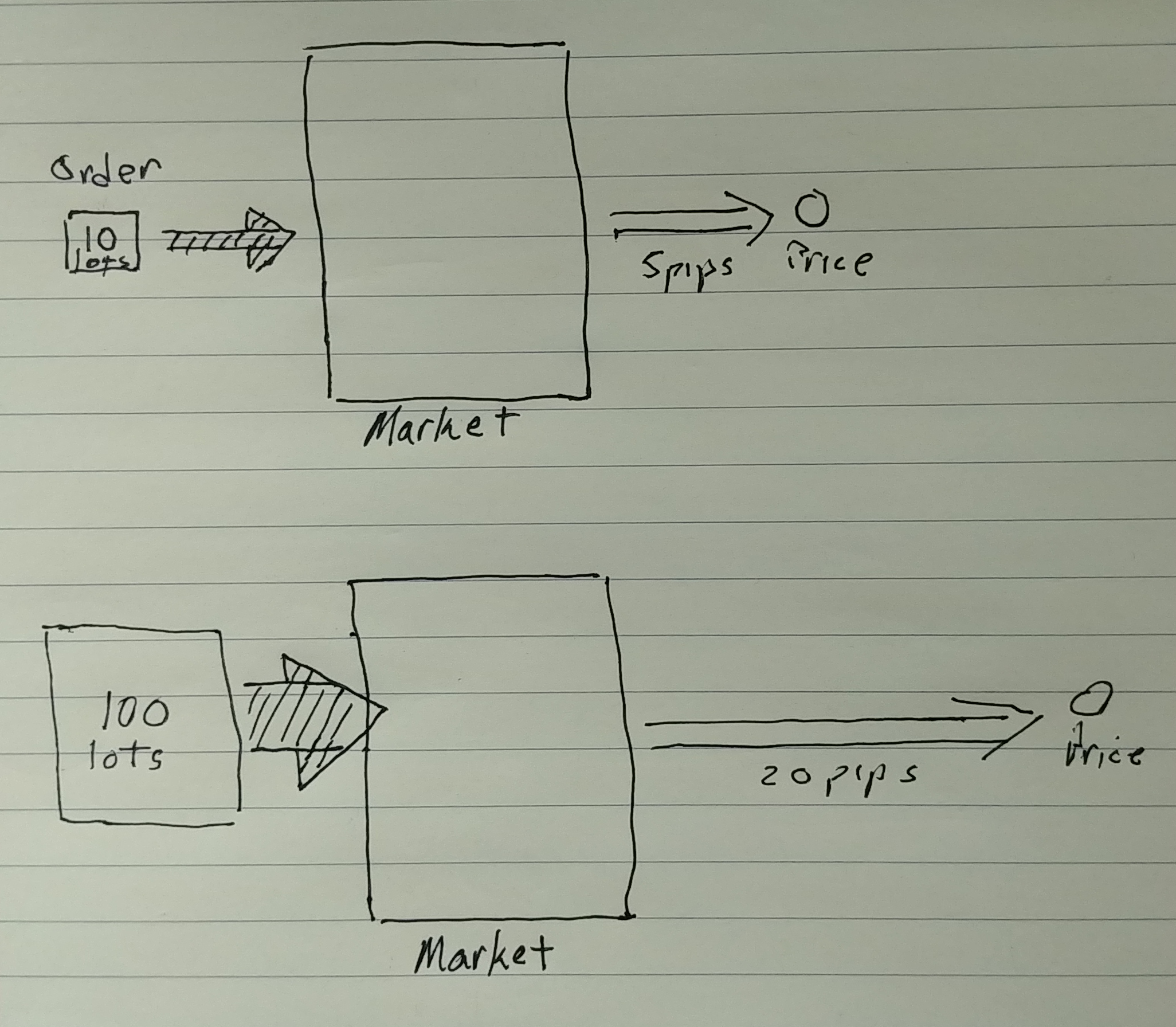
Effect Of Order Size On Price

What this information provides for us is a probabilistic confidence of determining if a trade is entered that it either will or it will not continue on toward an identified profit target.

Whether it reaches that profit target or not is another issue.

For a simple discussion of this, we turn to Newton's Second Law of Motion which states:

"Newton's second law is a quantitative description of the changes that a force can produce on the motion of a body.

It states that the time rate of change of the momentum of a body is equal in both magnitude and direction to the force imposed on it.

The momentum of a body is equal to the product of its mass and its velocity. Momentum, like velocity, is a vector quantity, having both magnitude and direction. A force applied to a body can change the magnitude of the momentum, or its direction, or both.

Newton's second law is one of the most important in all of physics. For a body whose mass m is constant, it can be written in the form F = ma, where F (force) and a (acceleration) are both vector quantities."

REF: Encyclopaedia Britannica: Newton's laws of motion

Two concepts are mentioned here. First is momentum (usually, p), and Second is force (F).

An object, let's just call it the price, has momentum (p) because it is being moved. I'm going to propose then that 'the market' (which are traders placing orders) is the force (F) acting on the price to give that price momentum.

A trader who inputs a large lot size order applies more force at the price, i.e. will move that price further because of the size of that order, than a small lot size order. I showed that in the last diagram.

The force of the order creates momentum in the price, i.e. the price moves strongly in the direction of the order - let's say long. However, unless many other traders are making long trades, or there was only that one large order, then price will start to slow down.

The below diagram shows the opposite of that, i.e. when there is momentum behind the price because of continuous order flow pushing price.

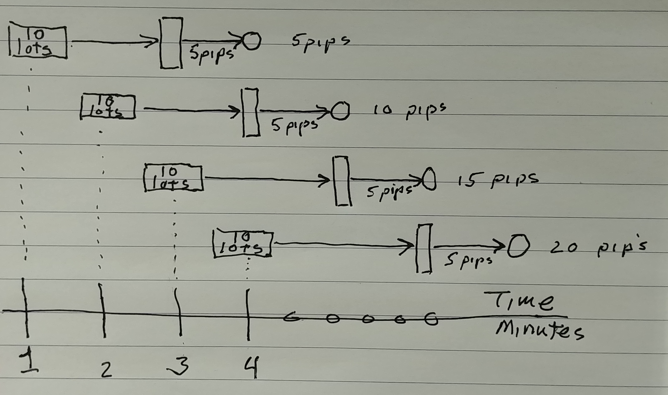
Effect Of Continuous Order Flow On Price

As you can see, continuous 10 lot orders are placed over time with each order adding, so-to-speak, momentum to the price whick keeps it moving toward the profit target. That's when there is momentum to price.

Thus the reverse is true. Price can slow down either because there are no other large long orders being placed, or because there are many more short orders being placed that create the overall market sentiment to change to short bias.

The longer price receives reduced force from further large orders, or encounters resistance from short orders the less likely it is to be able to have the momentum to continue toward the trader's intended profit target.

A trader evaluating this situation would thus like to know, or at least better understand, the overall state of the system, i.e. the market, before entering a long trade.

And this brings us not only back to the study of the market as a system defined by Brownian Motion, but also a statistical model that has been defined in what's called the Black-Scholes Options Pricing Model.

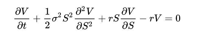
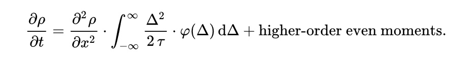
Equation for the Black-Scholes Options Pricing Model

Unfortunately, because the creators of the Black-Scholes Options Pricing Model had most likely only derived the model from Brownian Motion structure, and had not considered true market force risk, it was one of the major reasons the entire derivatives market imploded in 2008 creating the greatest economic collapse and recession since we've had post The Great Depression.

Long-Term Capital Management was a hedge fund based in Greenwich, Connecticut that used absolute return trading strategies combined with high financial leverage. LTCM was founded in 1994 by John Meriwether, the former vice-chairman and head of bond trading at Salomon Brothers, with principle board members Myron S. Scholes and Robert C. Merton.

LCTM was initially successful with annualized return of over 21%, 43%, and 41% in the third year. However, in 1998 it lost $4.6 billion in less than four months due to a combination of high leverage and exposure to the 1997 Asian financial crisis and 1998 Russian financial crisis, and collapsed in the late 1990s.

The reason I mention all of this is because the Black–Scholes Options Pricing Model was originally used to evaluate the price of a stock option as a function of the time remaining until the option expiration date.

What this means is that if the price of the underlying stock either decreases or even remains the same, then a call (long/buy) option's value would decrease as the expiration date got closer. That's time decay of the option.

The following 2 rough drawings basically illustrate this. The stock price is the dark heavy line, and the lighter dotted line represents the option. The example is for an XYZJune50 call, i.e. the option purchased for $1 at a stock price of $20 should be worth $5 if the stock price reaches $50 by June.

The first diagram shows the option price as a function of stock price when the stock does hit $50 by the target date, whereas the option price rapidly decays to zero when the underlying stock fails to reach $50 by the target date.

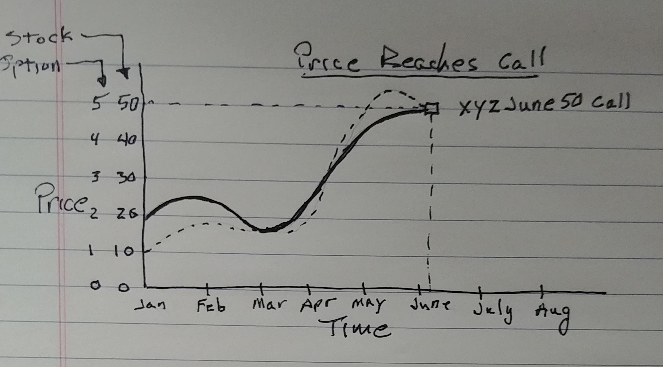
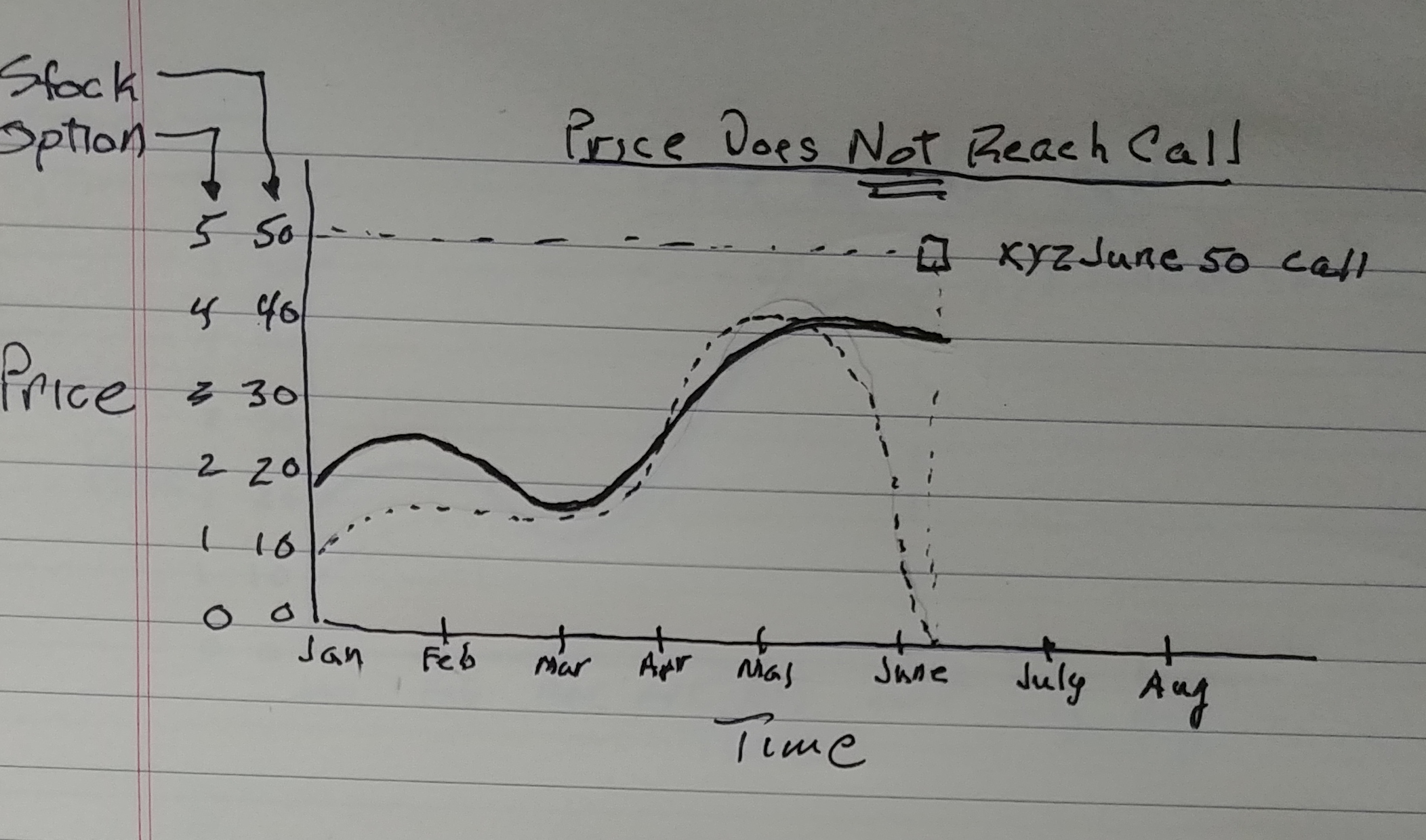
Though far from exact, the diagrams demonstrate the exponential decay of the option regardless of the rather stable movement of the stock even though not continuing toward the strike price still weeks away. The Black-Scholes equation was used similarly in derivatives trading to calculate the estimated value over time. Whereas the process may work for options, the calculations for derivatives fell far short of determining the real risk of the positions.

Mapping that equation into the pricing of financial derivatives, particularly in the pricing of individual tranches of mortgage backed securities, was a huge error in misjudging the underlying risk. Thus, as these securities lost value, the equation failed to correctly identify the increasing risk of more securities losing value as time moved forward, thus creating a rapid (4 month) implosion of not only LCTM, but most of our financial system.

In currency trading, the longer price fails to move rapidly, i.e. has momentum, toward the profit target the underlying probability that price will reach that target decays. The trick then is in determining the momentum of price as a function of time.

If you're looking at a profit target 20 pips away, and current price action on a 15 minute time frame has an ATR of 20, then the theoretical answer is 15 minutes, right?

Well, almost.... That would be the case as long as each candle was stacked close-to-open without retracement below the previous candle's close. However, to simplify the discussion, I'm just going to ignore that, and propose the 'happy path' time to profit target as 15 minutes.

If I was looking at this same situation from the stand point of the 5 minute time frame which (conveniently) has an ATR of 5 pips, then you'd still get the same time of 15 minutes to profit target, it's just that it's going to take 3 of those 5 minute candles to get there.

It would appear that it's immaterial whether you're looking at the 15 minute or the 5 minute time frame because either the price will get to the profit target in 15 minutes, or it won't.

And though that's true, if you're actually trading on the 5 minute time frame, and if price staggers during that second, five minute candle, you would have an indication that perhaps price does not have enough momentum to make it all the way to the profit target. In the first candle, price went 5 pips. Great. But in the second candle, price retreated 5 pips, and is basically back to its trade entry location. Hummmm....

And what does that mean? Well, it means that if price is going to get to the profit target 20 pips away instead of being only 5 pips away, that it is going to have to have some enormous input of force to it to drive it 20 pips now in 5 minutes, i.e. the distance the last 5 minute candle would have had to travel if the second candle had advanced 5 pips instead of dropping 5 pips.

Because the distance to the profit target has increased, if there is no increase in momentum, i.e. momentum decays, then the risk increases.....

But isn't the risk increasing the same if you're monitoring price on the 15 minute time frame? Of course it is.

You just don't... see... it....

But the risk is increasing, none-the-less....

And so the question you have to ask yourself if you are able to perceive this decay of momentum and thus increase in risk when trading on higher time frames: Is this information relevant or important to you?

If the information is important to you, then you need to understand exactly what price action time decay is, and how to implement that into the position risk management of your trading.

Video: 4 Methods of FOREX Entry Risk Analysis

Video: Risk Management

Video: Close FOREX Currency Trades Based On Risk Not Profit

Video: Close Trades When Price Momentum Changes

Video: Problems With Using Technical Analysis in FOREX Trading

Video: Fallacy of FOREX Trading Indicator Confluence